time_series_vis

Module: missions.nodes.visualization.time_series_vis

Visualize data in time-amplitude or time-frequency representations

This module contains nodes that can be used to visualize the data as time series. All these nodes use the functionality of the VisualizationBaseNode.

Inheritance diagram for pySPACE.missions.nodes.visualization.time_series_vis:

Class Summary

TimeSeriesPlotNode([channel_names, ...])	A node that allows to monitor the processing of time series
SpectrumPlotNode([channel_names, colorbar, ...])	Construct spectrogram of the data using FFT
ScatterPlotNode(plot_ms[, channels])	Creates a scatter plot of the given channels for the given point in time
HistogramPlotNode(plot_ms, value_range[, ...])	Creates a histogram of the given channels for the given point in time

Classes

TimeSeriesPlotNode

class pySPACE.missions.nodes.visualization.time_series_vis.TimeSeriesPlotNode(channel_names=None, separate_channels=False, class_difference=False, **kwargs)

Bases: pySPACE.missions.nodes.visualization.base.VisualizationBase

A node that allows to monitor the processing of time series

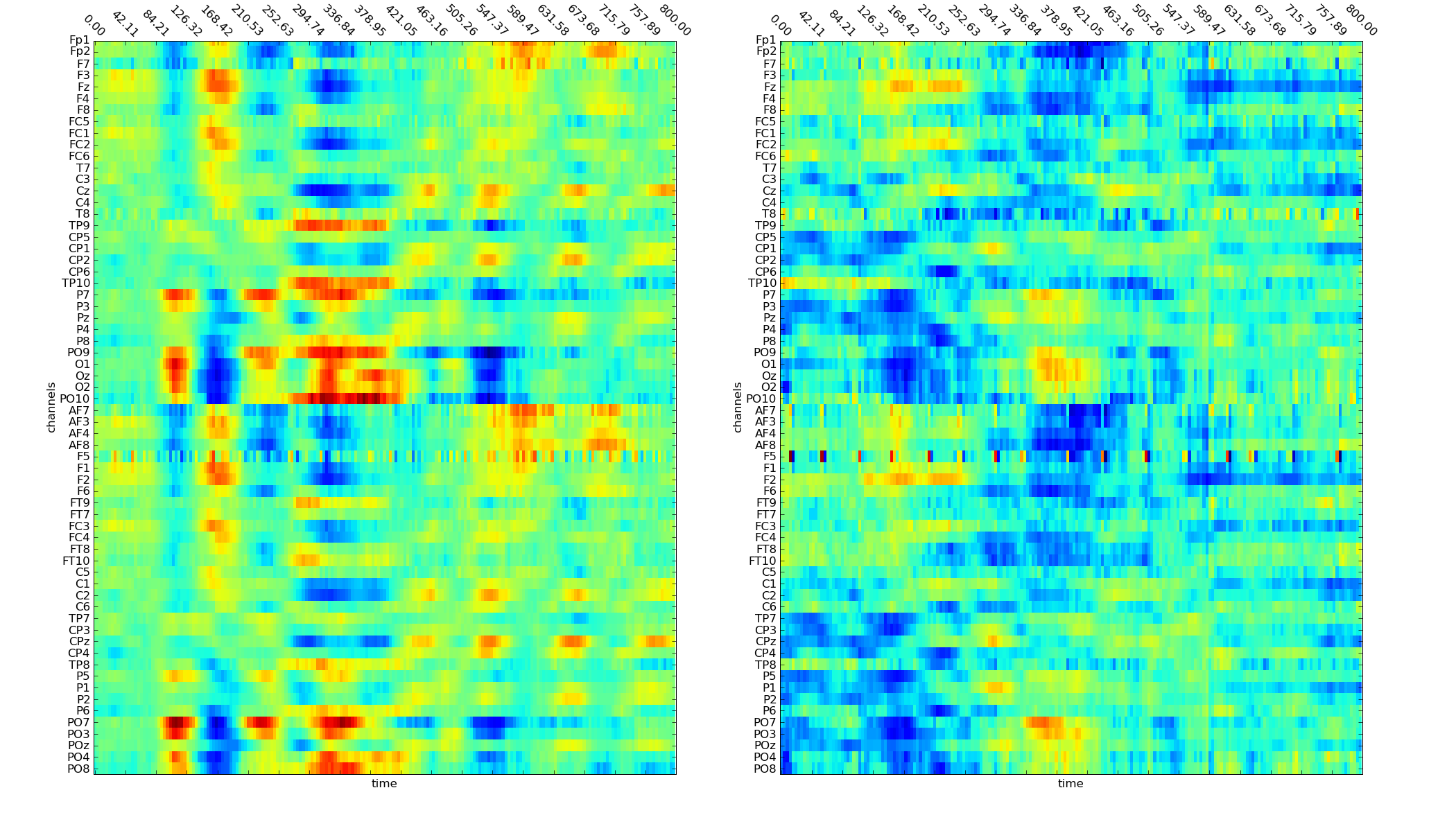
This node plots the time series data either in one column for all channels or for a single selected channel. The node inherits the functionality of the VisualisationBase.

See documentation of VisualisationBase to view basic functionality. If not specified differently using the parameters below, the data is plotted in one matrix for each class (using pylab.matshow).

Parameters

channel_names:

If one channel_name is given, only information about this channel is plotted. If more channels are specified, they are plotted separately in one subplot (forces separate_channels to True).

(optional, default: None)

separate_channels:  

Each channel gets a separate subplot (amplitude vs time), either arranged in rows and columns or arranged according to position on the head (see parameter physiological_arrangement in base class). (optional, default: False)

class_difference:  

If this is True, the created plot shows the difference between the two classes. This option only works if 2 classes are present at the same time! (optional, default: False)

Exemplary Call

-
     node : Time_Series_Plot
     parameters :
          averaging : True
          online : True
          separate_channels: True

Author:

Sirko Straube (sirko.straube@dfki.de)

Date of Last Revision:  

2012/12/21

POSSIBLE NODE NAMES:  

• Time_Series_Plot
• TimeSeriesPlot
• TimeSeriesPlotNode

POSSIBLE INPUT TYPES:  

• TimeSeries

Class Components Summary

_plotValues(values, plot_label, fig_num[, ...])
_plot_all_channels(data, tpoints, channel_names)
_plot_all_channels_separated(tpoints, values)	This function generates time series plot separated for each channel
input_types
reset()	Reset the state of the object to the clean state it had after its

input_types = ['TimeSeries']

__init__(channel_names=None, separate_channels=False, class_difference=False, **kwargs)

reset()

Reset the state of the object to the clean state it had after its initialization

_plotValues(values, plot_label, fig_num, store_dir=None, counter=0)

_plot_all_channels(data, tpoints, channel_names)

_plot_all_channels_separated(tpoints, values)

This function generates time series plot separated for each channel

SpectrumPlotNode

class pySPACE.missions.nodes.visualization.time_series_vis.SpectrumPlotNode(channel_names=None, colorbar=False, NFFT=128, noverlap=0, **kwargs)

Bases: pySPACE.missions.nodes.visualization.base.VisualizationBase

Construct spectrogram of the data using FFT

This node uses the data for a power-spectral density (psd) computation plotted as time-frequency representation. The core function here is specgram from matplotlib.mlab. The node inherits the functionality of the VisualisationBase.

See documentation of VisualisationBase to view basic functionality.

If not specified differently using the parameters below, all channels are plotted in physiological arrangement separately for each class.

Note

If you average data, then the spectrogram is always computed on the average. Currently, the averaging of the power values is not implemented.

Parameters

channel_names:

All classes are plotted directly in one figure, if only one channel_name is specified (e.g., ‘Pz’). If more channels are specified, you get a plot of all channels for one class, i.e. for two classes two plots are returned. The default is that all channels are displayed which the user can explicitly specify using the keyword ‘all’.

(optional, default: None)

colorbar:

Determine if the colorbar should be displayed. Currently, the colorbar is switched off when parameter physiological_arrangement is True.

(optional, default: False)

NFFT:

The number of data points used in each block for the FFT. Must be even; a power 2 is most efficient.

(optional, default: 128)

noverlap:

The number of points of overlap between blocks of the FFT.

(optional, default: 0)

Exemplary Call

-
    node : Spectrum_Plot
    parameters :
        averaging : True
        online : True

Author:

Sirko Straube (sirko.straube@dfki.de)

Date of Last Revision:  

2013/01/18

POSSIBLE NODE NAMES:  

• SpectrumPlot
• Spectrum_Plot
• SpectrumPlotNode

POSSIBLE INPUT TYPES:  

• TimeSeries

Class Components Summary

_plotValues(values, plot_label, fig_num[, ...])
_plot_spectrum(data, sampling_frequency)
input_types

input_types = ['TimeSeries']

__init__(channel_names=None, colorbar=False, NFFT=128, noverlap=0, **kwargs)

_plotValues(values, plot_label, fig_num, store_dir=None, counter=0)

_plot_spectrum(data, sampling_frequency)

ScatterPlotNode

class pySPACE.missions.nodes.visualization.time_series_vis.ScatterPlotNode(plot_ms, channels=None, **kwargs)

Bases: pySPACE.missions.nodes.base_node.BaseNode

Creates a scatter plot of the given channels for the given point in time

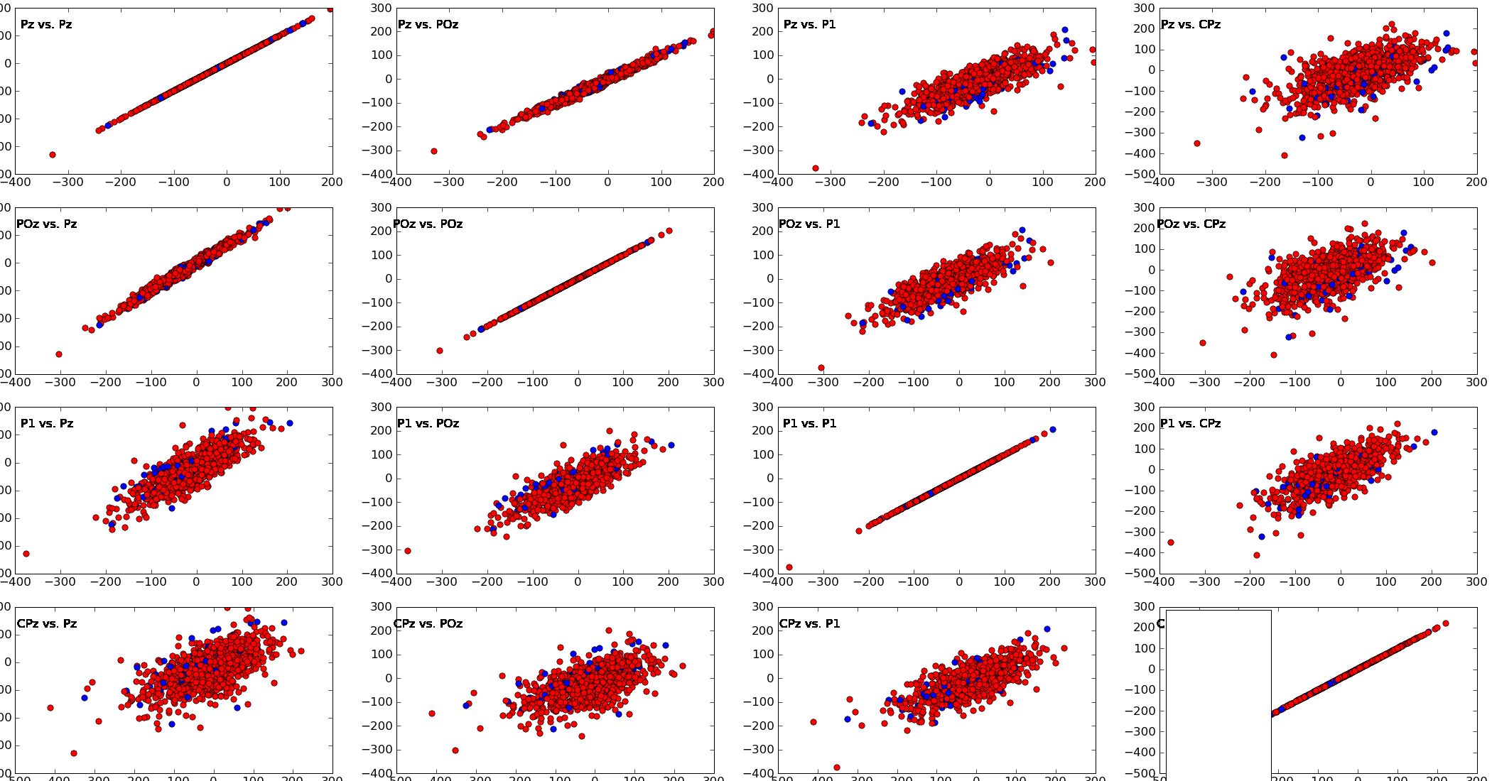
This node creates scatter_plot of the values of all vs. all specified channels for the given point in time (plot_ms).

Parameters

plot_ms:The point of time, for which the scatter plots are drawn. For instance, if plot_ms = 200, all the values of the selected channels are collected that were measured 200ms after the window start and the scatter plots for these values are drawn channels:If channels is not None, only scatter plots for these specified channels are plotted. If channels is not specified, scatter plots for the first 7 available channels are drawn.

Note

The maximal number of channels has to be less than 8 since more than a 7*7 matrix of plots is hard to get plotted into one window.

Exemplary Call

-   node : ScatterPlot
    parameters :
        plot_ms : 2

POSSIBLE NODE NAMES:  

• Scatter_Plot
• ScatterPlotNode
• ScatterPlot

POSSIBLE INPUT TYPES:  

• TimeSeries

Class Components Summary

_execute(data)
_stop_training([debug])
_train(data, label)	This node is not really trained but uses the labeled examples to generate a scatter plot.
figure_number
input_types
is_supervised()	Returns whether this node requires supervised training
is_trainable()	Returns whether this node is trainable.

input_types = ['TimeSeries']

__init__(plot_ms, channels=None, **kwargs)

figure_number = 0

is_trainable()

Returns whether this node is trainable.

is_supervised()

Returns whether this node requires supervised training

_train(data, label)

This node is not really trained but uses the labeled examples to generate a scatter plot.

_stop_training(debug=False)

_execute(data)

HistogramPlotNode

class pySPACE.missions.nodes.visualization.time_series_vis.HistogramPlotNode(plot_ms, value_range, channels=None, **kwargs)

Bases: pySPACE.missions.nodes.base_node.BaseNode

Creates a histogram of the given channels for the given point in time

This node creates histograms of the values of all specified channels for the given point in time (plot_ms). The value range is restricted to the specified value_range, values outside of this range are not plotted.

Parameters

plot_ms:The point of time, for which the histograms are drawn. For instance, if plot_ms = 200, all the values of the selected channels are collected that were measured 200ms after the window start and the histograms for these values are drawn value_range:A pair (tuple) that specifies the range of values that are plotted in the histogram. Values outside this range are not drawn. channels:If channels is not None, only histograms for these specified channels are plotted. If channels is not specified, histograms for all available channels are plotted.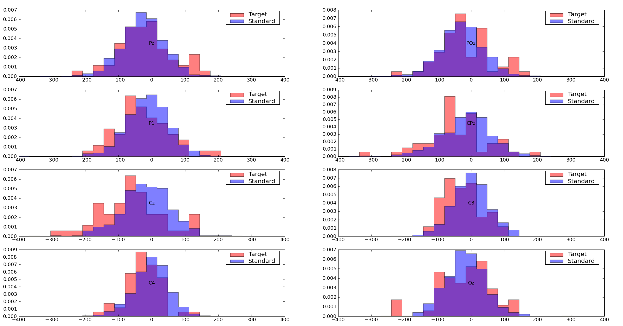

Exemplary Call

-
    node : HistogramPlot
    parameters :
        plot_ms : 2
        value_range : [-10, 10]

POSSIBLE NODE NAMES:  

• HistogramPlot
• HistogramPlotNode
• Histogram_Plot

POSSIBLE INPUT TYPES:  

• TimeSeries

Class Components Summary

_execute(data)
_stop_training([debug])
_train(data, label)	This node is not really trained but uses the labeled examples to
input_types
is_supervised()	Returns whether this node requires supervised training
is_trainable()	Returns whether this node is trainable.

input_types = ['TimeSeries']

__init__(plot_ms, value_range, channels=None, **kwargs)

is_trainable()

Returns whether this node is trainable.

is_supervised()

Returns whether this node requires supervised training

_train(data, label)

This node is not really trained but uses the labeled examples to generate a histogram

_stop_training(debug=False)

_execute(data)