Process EEG data (only) from within a Python session

In this tutorial we will learn how to use pySPACE from within a Python shell without explicitly using the whole functionality of pySPACE. Here, we get the “data pieces” from a pySPACE data generator with which we perform the specified node chain and get the results. Therefore, it has to be underlined that we still have to use a bit resources to provide the node chain with the correct data.

Prerequisites

Before we start, some prerequisites have to be fulfilled:

1. Download and install pySPACE as it is described here.

2. The example data can be found in the storage of the pySPACEcenter under eeg_examples. There you will find the Folder “test_data/Set1”. The node_chain and the windower file needed in this tutorial are located in the specs folder of the pySPACEcenter. These are two .yaml files named node_chains/example_tutorial_eeg_only.yaml and node_chains/windower/example_tutorial_eeg_only_window_spec.yaml

3. To make things easier, your PYTHONPATH variable should contain the path to pySPACE. E.g. consider your framework folder to be in “/home/user/software/”: You can either change your .bash_profile by adding:

   export PYTHONPATH=/home/user/software/:$PYTHONPATH
   

   or by starting your Python session (or script) with:

   import sys
   sys.path.append('/home/user/software/')
   

Data Inspection

The first step in every investigation is of course to get some knowledge about the data you are investigating. The test data is in the Set1 folder, stored in a binary .eeg file. It consists of 32-channels which all “measured” a sinusoid signal and you have two markers “R 32” and “R 64” in the data. Using an EEG file viewer as integrated in BESA (BESA GmbH), BrainVision Analyzer 2 (Brain Products GmbH) or EEGLAB, the data looks like this:

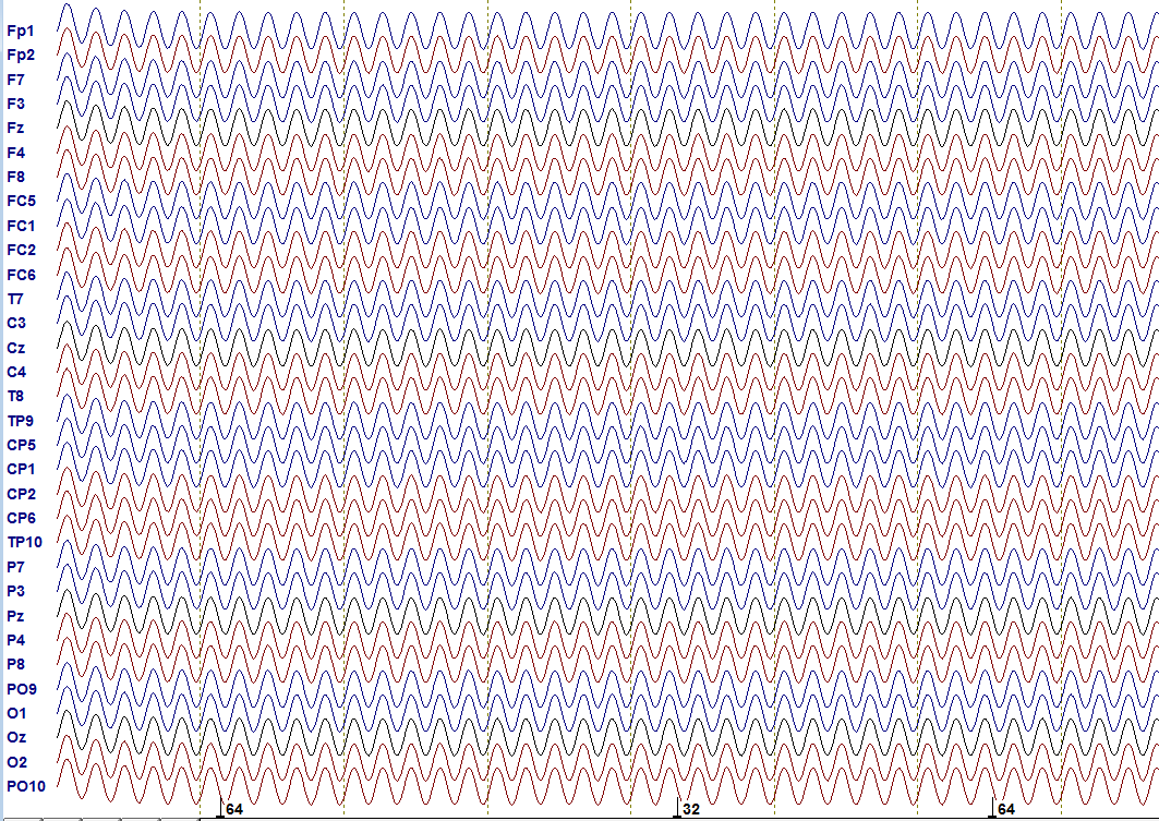
Test data: shown is the progress over time (time between dashed lines equals 1 second) including the channel names as they would occur in a real EEG experiment. Markers are illustrated at the bottom. They label important events.

Three other files exist in the data folder: The files ending with .vhdr and .vmrk directly belong to the .eeg file specifying additional information. In contrast to the actual data, they are not in a binary format, so you can open them with a text editor if you are curious. The vhdr-file contains general additional information and the vmrk file contains name and time point of the markers you see above.

The last file, named metadata.yaml is mandatory for loading data. It contains some general information (to get an idea of what you can specify in the metadata.yaml see here). The format of the file is YAML, which was developed as a human readable (i.e. in text format) data format. The YAML format is widely used in the software. For the moment, you do not need to care about the metadata.yaml, but its presence already indicates how the data will be loaded: with the help of pySPACE. More details on YAML can be found here.

Now let us look at the node chain and how to start it:

The First Node Chain

As introduced above, the files are located after installation in the specs folder of your pySPACEcenter. Relevant are the two YAML files: example_tutorial_eeg_only.yaml contains the processing sequence for the data and windower/example_tutorial_eeg_only_window.yaml contains some information how the data should be cut relative to the markers and how this data should be labeled. This file is only necessary here, because we are dealing with raw EEG data, which -as a first step- has to be windowed. You can open and look at it, the definitions are more or less self explaining (you can find a bit more information on windowing in the general node chain tutorial).

Now let us look at the processing sequence. If you open example_tutorial_eeg_only.yaml you will see the following:

- 
    node: Offline_EEG_Source
    parameters : 
        windower_spec_file : "/Users/sstraube/pySPACEcenter/specs/node_chains/windower/example_tutorial_eeg_only_window_spec.yaml"
        local_window_conf : True
-
    node : Detrending
    parameters:
        subset : eval(range(100,201))
- 
    node : Decimation
    parameters : 
        target_frequency : 100.0
        comp_type : normal
-
    node : FFT_Band_Pass_Filter
    parameters : 
        pass_band : [0.0, 10.0]
-   
    node : Time_Series_Sink

This is the node chain that defines how the data is treated. In every node, the data is processed and passed to the next node, until finished (for more information on available nodes see node documentation). Here, e.g., the data is detrended, its sampling frequency decimated and finally bandpass-filtered between 0 Hz and 10 Hz. The Source and Sink nodes deal with loading and saving of the data. By convention, when using launch in the run environment, every node chain should start with a source node and end with a sink node.

The path given here is just an example. Therefore, before executing, you should adjust the path of the windowing spec file according to your own.

Running the NodeChain

Now let us import the software and run the node chain! You can do the following either in a Python session or by writing and executing a script.

As a first step, we import everything that is necessary:

from pySPACE.environments.chains.node_chain import NodeChainFactory
from pySPACE.environments.chains.node_chain import BenchmarkNodeChain
from pySPACE.resources.dataset_defs.base import BaseDataset

The YAML file is converted to an executable NodeChain with the NodeChainFactory. The BenchmarkNodeChain was written to execute offline data and the resources package is used to collect the necessary information concerning the underlying data, i.e. the so called dataset.

Second, we define necessary directories and location of the NodeChain (please adjust the paths accordingly):

node_chain='/home/user/pySPACEcenter/specs/node_chains/example_tutorial_eeg_only.yaml'
data_dir='/home/user/pySPACEcenter/examples/storage/eeg_examples/test_data/Set1/'
store_dir='/home/user/pySPACEcenter/storage/myresults/'

The store_dir specifies where the data should be stored to disk. As a next step, we have to read the text from the YAML file:

pyspacespecfile=open(node_chain)
pyspacespec=pyspacespecfile.read()
pyspacespecfile.close()

Now a valid node chain is created with the given specifications. The necessary functions for execution are defined by the class in the module node_chains (in this case BenchmarkNodeChain). Here, you might get a warning which you can ignore.

my_flow = NodeChainFactory.flow_from_yaml(Flow_Class=BenchmarkNodeChain, flow_spec=pyspacespec)

As introduced above, the data is loaded with the help of resources and the corresponding metadata.yaml file. This is done in the next step:

input_dataset = BaseDataset.load(data_dir)

Now the data is processed and the result is stored in the variable result, which has a data type that is defined in pySPACE and comes with its own store method. By calling this method, the data is stored to disk in the appropriate data format:

result = my_flow.benchmark(input_collection = input_dataset, persistency_directory = store_dir, run=1)
result.store(store_dir)

In principle, you can use more than one set (=run) for your evaluation, but again you have to specify how to deal with these, e.g., how to deal with the numbering. As you already may have guessed, this is been shaded for the user when using the software. Thus, you should not worry about the argument run=1 for now.

Curious on what you have done?

Since you’ve seen already in the spec file how the data is processed, the answer might be a little bit disappointing: besides that it is windowed, the data is nearly the same. Nevertheless you can play around a bit with the stored data to get an idea of how it is generally stored as long as it is a TimeSeries. To do this, you can start with the following code in your store_dir and go on as you like...

import cPickle
import pylab as pl

data=cPickle.load(open('time_series_sp0_test.pickle'))
first_elem=data[0][0]

print first_elem.tag
print first_elem.channel_names

pl.plot(first_elem[:,0]) #plot data of first electrode
pl.show()