classification_performance_sink

Module: missions.nodes.sink.classification_performance_sink

Calculate performance measures from classification results and store them

All performance sink nodes interface to the metric datasets, where the final metric values . are calculated.

These results can be put together using the PerformanceResultSummary.

Inheritance diagram for pySPACE.missions.nodes.sink.classification_performance_sink:

Class Summary

PerformanceSinkNode([classes_names, ...])	Calculate performance measures from standard prediction vectors and store them
LeaveOneOutSinkNode([classes_names, ...])	Request the leave one out metrics from the input node
SlidingWindowSinkNode([uncertain_area, ...])	Calculate and store performance measures from classifications of sliding windows

Classes

PerformanceSinkNode

class pySPACE.missions.nodes.sink.classification_performance_sink.PerformanceSinkNode(classes_names=[], ir_class='Target', sec_class=None, save_individual_classifications=False, save_roc_points=False, weight=0.5, measure_times=True, calc_soft_metrics=False, sum_up_splits=False, dataset_pattern=None, calc_AUC=True, calc_loss=True, calc_train=True, save_trace=False, decision_boundary=None, loss_restriction=2, evaluation_type='binary', **kwargs)

Bases: pySPACE.missions.nodes.base_node.BaseNode

Calculate performance measures from standard prediction vectors and store them

It takes all classification vectors that are passed on to it from a continuous classifier, calculates the performance measures and stores them. The results can be later on collected and merged into one tabular with the NodeChainOperation. This one can be read manually or it can be visualized with a gui.

Note

FeatureVectorSinkNode was the initial model of this node.

Parameters

evaluation_type:  

Define type of incoming results to be processed. Currently binary (BinaryClassificationDataset) and multinomial (MultinomialClassificationDataset) classification (also denoted as multiclass'' classification) and ``regression (even for n-dimensional output) (RegressionDataset) metrics can be calculated.

For the multinomial and regression case several parameters are not yet important. These are:

• ir_class
• save_roc_points
• calc_AUC
• calc_soft_metrics
• calc_loss
• sum_up_splits

Warning

Multinomial classification and regression have not yet been used often enough with pySPACE and require additional testing.

(optional, default: “binary”)

ir_class:

The class name (as string) for which IR statistics are to be output.

(recommended, default: ‘Target’)

sec_class:

For binary classification the second class (not the ir_class) can be specified. Normally it is detected by default and not required, except for one_vs_REST scenarios, where it can not be determined.

(optional, default: None)

save_individual_classifications:  

If True, for every processed split a pickle file will be generated that contains the numerical classification result (cresult) for every individual window along with the estimated class label (c_est), the true class label (c_true) and the number of features used (nr_feat). The result is a list whose elements correspond to a single window and have the following shape:

[ [c_est, cresult, nr_feat], c_true ]

(optional, default: False)

save_roc_points:  

If True, for every processed split a pickle file will be generated that contains a list of tuples (=points) increasing by FP rate, that can be used to plot a Receiver Operator Curve (ROC) and a list, that contains the actually used point in the ROC space together with (0|0) and (1|1). The result has the following shape:

( [(fp_rate_1,tp_rate_1), ... ,(fp_rate_n,tp_rate_n)],
  [(0.0,0.0), (fp_rate, tp_rate), (1.0,1.0)])

For comparing ROC curves, you can use the analysis GUI (performance_results_analysis.py).

(optional, default: False)

weight:

weight is the weight for the weighted accuracy. For many scenarios a relevant performance measure is a combination of True-Positive-Rate (TPR) and True-Negative-Rate (TNR), where one of the two might be of higher importance than the other, and thus gets a higher weight. Essentially, the weighted accuracy is calculated by

If this parameter is not set, the value equals the balanced accuracy. In the case of multinomial classification, this parameter has to be a dictionary.

(optional, default: 0.5)

measure_times:

measure the average and maximum time that is needed for the processing of the data between the last sink node in the node chain and this node.

(optional, default: True)

calc_soft_metrics:  

integrate uncertainty of classifier into metric prediction value is projected to interval [-1,1]

(optional, default: False)

calc_train:

Switch for calculating metrics on the training data

(optional, default: True)

calc_AUC:

Calculate the AUC metric

(optional, default: True)

calc_loss:

Integrates the calculated losses into the final csv-file. (L1, L2), (LDA, SVM, RMM), (restricted, unrestricted) and (equal weighted, balanced) losses are calculated in all combinations, resulting in 24 entries.

(optional, default: True)

loss_restriction:  

Maximum value of the single loss values. Everything above is reduced to the maximum.

(optional, default: 2)

sum_up_splits:

If you use a CV-Splitter in your node chain, the performance sink adds up the basic metrics and calculates confusion matrix metrics with these values. The other metrics are averaged. So a lot of more testing examples are relevant for the calculation.

(optional, default: False)

dataset_pattern:  

If the __Dataset__ is of the form “X_Y_Z”, then this pattern can be specified with this parameter. The different values X, Y, Z will then appear in corresponding columns in the results.csv. Example: If the datasets are of the form “NJ89_20111128_3”, and one passes the dataset_pattern “subject_date_setNr”, then the results.csv will have the columns __Subject__, __Date__ and __SetNr__ with the corresponding values parsed (note the added underscores and capitalized first letter).

(optional, default: None)

decision_boundary:  

If your decision boundary is not at zero you should specify this for the calculation of metrics depending on the prediction values. Probabilistic classifiers often have a boundary at 0.5.

(optional, default: 0.0)

save_trace:

Generates a table which contains a confusion matrix over time/samples. There are two types of traces: short traces and long traces. The short traces contain only the information, if a classification was a TP, FN, FP or TN. The long traces furthermore contain loss values and are saved as a dictionary. To save only short traces (for, e.g. performance reasons), set save_trace to short. To save long and short traces, set save_trace to True. The encoding in trace is: :TP: 0 :FN: 1 :FP: 2 :TN: 3

(optional, default: False)

Exemplary Call

-  
    node : Classification_Performance_Sink
    parameters :
        ir_class : "Target"
        weight : 0.5

Input:

PredictionVector

Output:

ClassificationDataset

Author:

Mario Krell (mario.krell@dfki.de)

Created:

2012/08/02

POSSIBLE NODE NAMES:  

• Classification_Performance_Sink
• ClassificationSinkNode
• PerformanceSinkNode
• PerformanceSink

POSSIBLE INPUT TYPES:  

• PredictionVector

Class Components Summary

_train(data, label)
calculate_classification_trace(...[, ...])	Calculate the classification trace, i.e.
get_result_dataset()	Return the result dataset
input_types
is_supervised()	Return whether this node requires supervised training.
is_trainable()	Return whether this node is trainable.
process_current_split()	Main processing part on test and training data of current split
reset()	classification_dataset has to be kept over all splits
set_helper_parameters(classification_vector, ...)	Fetch some node parameters from the classification vector
store_state(result_dir[, index])	Stores additional information (classification_outcome, roc_points) in the result_dir

input_types = ['PredictionVector']

__init__(classes_names=[], ir_class='Target', sec_class=None, save_individual_classifications=False, save_roc_points=False, weight=0.5, measure_times=True, calc_soft_metrics=False, sum_up_splits=False, dataset_pattern=None, calc_AUC=True, calc_loss=True, calc_train=True, save_trace=False, decision_boundary=None, loss_restriction=2, evaluation_type='binary', **kwargs)

reset()

classification_dataset has to be kept over all splits

is_trainable()

Return whether this node is trainable.

is_supervised()

Return whether this node requires supervised training.

_train(data, label)

process_current_split()

Main processing part on test and training data of current split

Performance metrics are calculated for training and test data separately. Metrics on training data help to detect errors in classifier construction and to compare in how far it behaves the same way as on testing data.

The function only collects the data, measures execution times and calls functions to update confusion matrices.

set_helper_parameters(classification_vector, label)

Fetch some node parameters from the classification vector

classmethod calculate_classification_trace(classification_results, calc_soft_metrics=False, ir_class='Target', sec_class=None, loss_restriction=2.0, calc_loss=False, decision_boundary=0.0, save_trace=True)

Calculate the classification trace, i.e. TN,TP,FN,FP for every sample

The trace entries are encoded for size reasons as short (trace) or in a comprehensive version as dicts (long_trace)

The encoding in trace is:

TP:0 FN:1 FP:2 TN:3

Author:Hendrik Woehrle (hendrik.woehrle@dfki.de), Mario Krell (mario.krell@dfki.de) Returns:trace, long_trace

get_result_dataset()

Return the result dataset

store_state(result_dir, index=None)

Stores additional information (classification_outcome, roc_points) in the result_dir

LeaveOneOutSinkNode

class pySPACE.missions.nodes.sink.classification_performance_sink.LeaveOneOutSinkNode(classes_names=[], ir_class='Target', sec_class=None, save_individual_classifications=False, save_roc_points=False, weight=0.5, measure_times=True, calc_soft_metrics=False, sum_up_splits=False, dataset_pattern=None, calc_AUC=True, calc_loss=True, calc_train=True, save_trace=False, decision_boundary=None, loss_restriction=2, evaluation_type='binary', **kwargs)

Bases: pySPACE.missions.nodes.sink.classification_performance_sink.PerformanceSinkNode

Request the leave one out metrics from the input node

Parameters

see: PerformanceSinkNode

Exemplary Call

-  
    node : LOO_Sink
    parameters :
        ir_class : "Target"

POSSIBLE NODE NAMES:  

• LOO_Sink
• LeaveOneOutSinkNode
• LeaveOneOutSink
• LOOSink

POSSIBLE INPUT TYPES:  

• PredictionVector

Class Components Summary

process_current_split()

Get training results and input node metrics

process_current_split()

Get training results and input node metrics

SlidingWindowSinkNode

class pySPACE.missions.nodes.sink.classification_performance_sink.SlidingWindowSinkNode(uncertain_area=None, sliding_step=50, save_score_plot=False, save_trial_plot=False, save_time_plot=False, determine_labels=None, epoch_eval=False, epoch_signal=None, sort=False, unused_win_defs=[], **kwargs)

Bases: pySPACE.missions.nodes.sink.classification_performance_sink.PerformanceSinkNode

Calculate and store performance measures from classifications of sliding windows

This node inherits most of its functionality from PerformanceSinkNode. Thus, for parameter description of super class parameters see documentation of PerformanceSinkNode.

Additionally the following functionality is provided:

1) The definition of uncertain areas, which are excluded in the metrics calculation process, are possible. This is useful for sliding window classification, i.e. if the true label is not known in each sliding step. 2) It is possible to label the test data only now. For that an epoch signal (e.g. a movement marker window) must be specified. 3) Instead of excluding sliding windows from classifier evaluation, the ‘true’ label function shape (a step function, which is zero for the negative class and one for the positive class) can be somehow fit in the uncertain range. At the moment there is only one way for doing this:

• from_right_count_negatives: Find the point where prediction of the

  negative class starts by searching backwards in time. There can be specified how many ‘outliers’ are ignored, i.e. how stable the prediction has to be.

Parameters

uncertain_area:

A list of tuples of the lower and the upper time value (in ms) for which no metrics calculation is done. The values should be given with respect to the last window of an epoch, i.e. sliding window series (which has time value zero). If additionally determine_labels is specified then the first tuple of uncertain_area describes the bounds in which the label-change-point is determined. The lower bound should be the earliest time point when the detection makes sense; the upper bound should be the earliest time point when there MUST BE a member of the positive class.

(optional, default: None)

sliding_step:

The time (in ms) between two consecutive windows.

(optional, default: 50)

determine_labels:  

If specified the label-change-point (index where the class label changes from negative to positive class) is determined for every epoch. This is done via counting the occurrence of negative classified sliding windows from the index point where the positive class is sure (uncertain_area[1]) to the index point where the negative class is sure (uncertain_area[0]) If determine_labels instances were found in consecutively windows the label-change-point is has been reached. If determine_labels > 1, the methods accounts for outliers.

Note

Using this option makes it hard to figure out to which true class errors pertain (since it is somehow arbitrary). You should be careful which metric you analyze for performance evaluation (different class instance costs can’t be modeled).

epoch_signal:

The class name (label) of the event that marks the end of an epoch, e.g. the movement. This can be used when null_marker windows (of an unknown class) and a signal window which marks the event were cut out. With respect to this event the former windows will be relabeled according to classes_names.

(optional, default: None)

epoch_eval:

If True, evaluation is done per epoch, i.e. per movement. Performance metrics are averaged across epochs for every split. This option might be necessary if the epochs have variable length, i.e. the class distribution alters in every epoch.

(optional, default: False)

save_score_plot:  

If True a plot is stored which shows the average prediction value against the time point of classification.

(optional, default: False)

save_trial_plot:  

If True a plot is stored which shows developing of the prediction scores for each single trial.

(optional, default: False)

save_time_plot:

If True a plot is stored which shows the predicted labels for all trials across time.

(optional, default: False)

sort:

If True the data has to be sorted according to the time (encoded in the tag attribute. Be aware that this only makes sense for data sets with unique time tags.

(optional, default: False)

unused_win_defs:  

List of window definition names which shall not be used for evaluation.

(optional, default: [])

Exemplary Call

-  
    node : Sliding_Window_Performance_Sink
    parameters :
        ir_class : "LRP"
        classes_names : ['NoLRP','LRP']
        uncertain_area : ['(-600,-350)']
        calc_soft_metrics : True
        save_score_plot : True

Input:

PredictionVector

Output:

ClassificationCollection

Author:

Anett Seeland (anett.seeland@dfki.de)

Created:

2011/01/23

POSSIBLE NODE NAMES:  

• Sliding_Window_Performance_Sink
• SlidingWindowSinkNode
• SlidingWindowSink

POSSIBLE INPUT TYPES:  

• PredictionVector

Class Components Summary

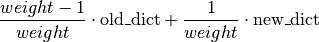
combine_perf_dict(old_dict, new_dict, weight)	Combine the values of the dicts by a weighting (iterative) average
from_right_count_negatives(y, target_number, ...)	Go through the bounded y (reverse) and find the index i, where target_number values have been consecutively the negative class.
get_result_metrics()	Calculate metrics based on evaluation type
process_current_split()	Compute for the current split of training and test data performance one sliding windows.
store_state(result_dir[, index])	Stores additional information in the given directory result_dir

__init__(uncertain_area=None, sliding_step=50, save_score_plot=False, save_trial_plot=False, save_time_plot=False, determine_labels=None, epoch_eval=False, epoch_signal=None, sort=False, unused_win_defs=[], **kwargs)

process_current_split()

Compute for the current split of training and test data performance one sliding windows.

get_result_metrics()

Calculate metrics based on evaluation type

from_right_count_negatives(y, target_number, bounds)

Go through the bounded y (reverse) and find the index i, where target_number values have been consecutively the negative class. Return i+target_number as critical index point (labels change)

combine_perf_dict(old_dict, new_dict, weight)

Combine the values of the dicts by a weighting (iterative) average

store_state(result_dir, index=None)

Stores additional information in the given directory result_dir